Part 1: Realistic Scenarios Require Accurate Modeling (Success Impaired: S&OP Technology Pitfalls)

This is where most problems with supply chain planning systems begin–particularly for production scheduling and S&OP/IBP solutions. To better illustrate where problems and confusion seep in, let’s look at what these systems typically look like in terms of (a) architecture & vendor offerings and (b) the actual production environments vs. solution models and how the two work together.

Architecture and Vendor Offerings

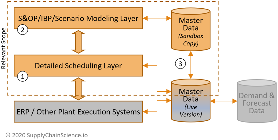
Architectures for most supply chain planning & scheduling technologies that support S&OP/IBP and production scheduling are divided into two solution layers and two mirrored sets of master data as depicted in Diagram 1.1.

Diagram 1.1: Typical Supply Chain Planning System Architecture

Demand forecasting (including collaborative forecasting, predictive forecasting, and advanced demand sensing technologies) provides an important input to S&OP/IBP and production planning processes and systems—the quality of this input can tremendously help or hinder business results. However, demand forecasting solutions have no bearing on the actual design or fit of the production model contained within the detailed scheduling and S&OP/IBP/scenario modeling layers which is the source of the problems described in this article. Given that, I am limiting the scope of this article to the design and fit of those production models and the scheduling and SOP/IBP/scenario modeling systems in which they reside. Subsequent articles will cover demand forecasting processes, tools, and technologies in greater detail.

Basic Architecture Components

(1) The Detailed Production Scheduling Layer incorporates into its logic all operating constraints, sequencing/routing options, and other choices required to drive the detailed schedule creation and execution of the eventual plan. It communicates with ERPs and plant execution systems to drive the material, production, and logistics processes as required to execute the implemented S&OP/IBP plan. This layer is the closest to the ERP and plant execution systems, and it draws upon the same master data that the ERP uses to run day-to-day operations.

(2) The S&OP/IBP/Scenario Modeling Layer mirrors all of the constraints contained in the detailed scheduling layer and relies on this “sandbox” copy to mimic all the constraints, sequencing/routing options, etc. The production model is a mirror of the one in the production scheduling/execution layer but with added functionality to support scenario modeling and what-if analyses included in S&OP/IBP processes and other decision-making exercises. This sandbox copy enables users to model and experiment with different scenarios without affecting live operations. Only when a user commits to a plan does the S&OP/IBP layer send that plan to the detailed scheduling layer for implementation. The detailed scheduling layer then sends the updated schedules, priorities, and other relevant information to the ERP and other plant execution systems as necessary.

(3) The Master Data contains the variable data that supports the ERP, detailed scheduling layer, and S&OP/IBP/scenario modeling layers. This includes forecasts, orders, bills of materials, costs, etc. as well as variable data associated with the production model. Consider the model within the detailed scheduling and S&OP/IBP layers as a mathematical equation that represents the plant, but that equation contains unresolved variables in place of many numeric values. In this analogy, the Master Data supplies the variable data required for the completion of the equation, and together they form the production model. A “live” version of master data supports day-to-day plant operations and is extensively used by the ERP, plant execution systems, and the detailed scheduling layer. Meanwhile, the S&OP/IBP/scenario modeling layer establishes a robust “sandbox” copy of relevant master data to enable users to model scenarios, what-ifs, and perform other inquiries without affecting actual operations.

Not all technology vendors offer each of these different layers, but each layer can be supplied by the same or different technology vendors. Large ERP providers like SAP and Infor offer all three components. Smaller pure-play S&OP/IBP solution providers may offer both the detailed scheduling layer and the S&OP/IBP/scenario modeling layer or just one of the two. I provide a few examples in Diagram 1.2 to illustrate variability among vendors.

Diagram 1.2 – Select Vendor Solutions by Layer

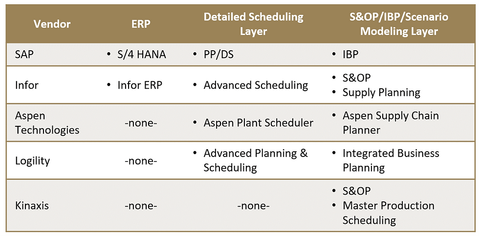
Diagram 1.2 Notes:

(1) The vendors for each layer are technically interchangeable. While it is common for some IT departments to seek offerings from the same vendor (usually oriented around their ERP vendor), that is not a technological or operational necessity. The layers communicate or “integrate” with each other and master data sets in much the same way whether a single vendor or multiple vendors provide the solutions. There can be value in having the detailed scheduling layer and S&OP/IBP layer provided by the same vendor as synchronization of the production models between those two layers is essential. However, it is not impossible to achieve this with separate vendors.

(2) The fact that a vendor does not have an offering in one or more columns does not necessarily make their available solution weaker and the fact that a vendor has offerings in all three columns does not necessarily make their solution any more capable. The capabilities and limitations are entirely within the respective solution’s design and functionality.

(3) In the rightmost column (S&OP/IBP/Scenario Modeling Layer), I limited the named applications to those that provide S&OP/IBP or production planning modules because the constraints, models, and optimization approaches, as discussed in this article, will function inside these applications. Many vendors also have offerings addressing demand planning, inventory planning, and other supply chain functions, but those applications are not central to the modeling and optimization challenges discussed in this article and therefore are not listed.

(4) SAP at one time offered its detailed scheduling layer known as Production Planning/Detailed Scheduling (PP/DS) as a separate application, but it now comes as an included component within S/4 HANA, SAP’s newer ERP offering.

(5) Kinaxis’ Master Production Scheduling module balances production allocations among two or more plants but it does not create detailed production schedules for a given plant. Therefore, this solution is more closely related to an S&OP/IBP/scenario modeling layer than a detailed scheduling layer and is listed accordingly.

This simplified table only lists five examples out of dozens of supply chain planning technology vendors to illustrate the relevant modules offered by each vendor. When the full range of vendors is considered, the complexity and ability to discern differences between vendors only becomes more challenging. The specific capabilities within each module add another layer of complexity as some modules complement a given functionality while other modules would overlap that same functionality. It can be a daunting task for buyers not already familiar with these vendors and modules to sort through all options from scratch and make an informed decision, so it’s understandable that many buyers rely on Magic Quadrants and similar reviews to shorten the list of options and simplify their selection process.

The proliferation of options is not a technological barrier itself, but it can introduce complexity early in a technology selection process. While the number of vendors and options is notable, it is still incidental to the main issue. To further drill down on the issue, let’s examine the two layers within the architecture that are to supply chain planning and optimization—the detailed scheduling and S&OP/IBP/scenario modeling layers—and what happens within them.

Actual Production Environments vs. Solution Models

In most cases, a production model will exist in the detailed scheduling layer solution and propagate “up” to the S&OP/IBP layer. Recall that the production model is comprised of software logic and master data that together create a systematic representation of the production process. It is this model that enables users to plan and schedule production, create hypothetical scenarios, and view the operational and financial impact of those scenarios.

It is not impossible, albeit relatively rare, that a highly accurate and detailed S&OP/IBP solution exists with no detailed scheduling layer solution at all. This is rare because detailed scheduling layer solutions are functionally closer to actual production execution and, by necessity, model the production process and constraints accurately as the solution can accommodate. Significant flaws in the detailed production scheduling model will result in rapid feedback in the form of production problems highlighted during the solution testing phase or, in some unlucky cases, during actual operations where these significant flaws would quickly impair actual production. An S&OP/IBP layer solution absent a detailed scheduling layer could, in theory, contain a full and perfectly accurate production model. But it will most likely have limitations or flaws as it is high-level or hypothetical and, in isolation, cannot be truly tested in the real production process.

Earlier, I used the analogy of a math equation with variables to describe the relationship between the production model contained within the detailed scheduling and S&OP/IBP/scenario modeling layers and the separate master data sets. The main parameters of the production model (i.e. the equation with unresolved variables) are defined in the detailed scheduling and S&OP/IBP/scenario modeling layers. The master data set supplies the variable data which is used by the production model to complete the “equation” and deliver a comprehensive and realistic result given actual factors, time, etc. of the modeled production process and its inputs and dependencies.

The technology that runs the detailed scheduling and S&OP/IBP/scenario modeling layers defines the structure of the constraints it can accept as well as the content and structure of the master data that it uses. Likewise, the core software/logic that drives the respective solutions are responsible for the modeling limitations referred to within this article, and these limitations are not correctable by a configuration adjustment or by enhancing master data quality. Conversely, when a detailed planning or S&OP/IBP layer solution can adapt to the enhancements in the quality or availability of master data, that is a desirable condition as it aligns with the typical evolution of an organization’s level of supply chain excellence. To better compare and contrast the two situations, let’s look at them more closely:

A. User-Driven Limitation: System Adapts As Manufacturer Capability Improves

A manufacturer may not yet have a full set of data representing all the changeover times and costs for a given production point or that manufacturer may not have a firm handle on the ratio of, say, heat and water content to cook time in a case where a naturally occurring substance is cooked in the production process. In this situation, the manufacturer can substitute approximate data or configure the point as a pass-through having the system ignore it until they arrive at a better, more accurate set of data and are ready to address it later. The model is technically limited by the missing or low-quality variable data at first, but that is a user-driven limitation and the manufacturer can upgrade the data at a time of their choosing as their process knowledge and modeling sophistication grows and without changing the technology. Over time, the manufacturer might iteratively supersede prior data sets with better and more expansive data resulting in more comprehensive models and higher fidelity results until the manufacturer effectively has a high-level “digital twin” of their production process.

B. System-Driven Limitation: No Fix Without Switching To A Different Technology

The problem addressed in this article is this opposite situation. The technology for a given layer is built using software code and data structures that are over-simplified and are not capable of accurately replicating the sophistication of the constraints and options within the production environment. Upon implementation, the manufacturer's model and data structures may be simplified (or dumbed down) to the level of the technology thus missing key constraints or options that exist in reality. These limitations could occur anywhere in the production process, but they will most often manifest at points with more complex constraints or those with numerous, conditional options. The manufacturer cannot “grow into” such a system as they are already hitting a hard limitation from the start. These limitations will also eventually impede the supply chain organization’s ability to evolve and restrict the operational and financial benefits that the manufacturer can attain.

The production models contained within the detailed scheduling layer solution should be as accurate as possible, with no fewer and no more constraints or options than exists given real operational limitations and flexibility. If excessive or artificial constraints are introduced, the planning/scenario modeling logic will not account for all possibilities and the results provided will already be sub-optimized (i.e. other potentially more optimal possibilities will be overlooked). Conversely, when the production model contains too few constraints or the system is incapable of accurately accounting for them, the scenario modeling and scheduling process can provide scenarios and schedules that are unrealistic. This is where most solutions begin to falter in ill-fitting environments—the solution is inherently incapable of accurately accounting for certain constraints, so the production model doesn’t address them which results in too few constraints out of the box even after configuration. But that’s the way the problem typically begins, what users experience is a little different. This is how it unfolds:

If a buyer chose such an ill-fitting solution and nothing was done to account for the missed constraints, the solution would regularly produce inexecutable results which would be a glaringly obvious failure. That’s clearly an unacceptable result, so what most often occurs, in this case, is the inherent inability to accurately model one or more given constraints is plugged with an artificial piece of logic, pseudo-constraints, or a configuration hack (i.e. an adaptation) that forces the solution to provide results within the range of possible operations without fully or accurately representing the limitations or flexibility of that constraint. To be clear, such adaptations should not be considered a normal configuration as they are the technical equivalent of duct tape and bubble gum. Significant adaptations are sometimes presented as a necessary customization, but also seen them referred to as configurations.

After these adaptations are applied, the resulting production model is either over-constrained, inflexible, or both, as compared to the manufacturer’s possible range of operations. But because “typical” operations at the time of implementation are accommodated in the adaptation, stakeholders may not discover this limitation until months or years later when a user attempts to model or implement a scenario that relies on a different set of circumstances or a different pass through that inadequately modeled constraint. Other stakeholders may notice it right away and simply try to work around it. The bottom line is that the adaptation, which was effectively a plug from the beginning, once again cannot adequately model the desired conditions. Diagrams 1.3 and 1.4 use a visual analogy to help illustrate these this concept.

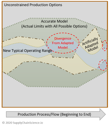
Diagram 1.3 – Production Options & Limits: Ill-Fitting Technology Best Case Upon Implementation

In this analogy, the entire square (grey) represents all unconstrained production options where a production process moves from left to right.

The green dotted line and area within represents the actual production limits considering all sequences, paths, routings, permutations, limitations, constraints, and flexibility (referred to collectively as “options”). Any plan that is realistically executable must fall within this green area.

In an ideal case, a solution’s production model design constrains the range of options such that they follow the green dotted lines exactly, no less and no more. It is then up to the solution’s solver approach and optimization logic to determine the best “path” given the full range of feasible options represented by the green area.

While most manufacturers have a large number of possible production options, they typically use a smaller set of options on a regular basis. This is because some options within the green area are clearly suboptimal or undesirable even if they are technically possible. We can say that the 80/20 rule applies where only 20% of all possible production options account for 80% (or more) of production options that a manufacturer uses over a given timeframe. This smaller range of “typical” operations is represented by the typical operating range in blue.

With an ill-fitting solution, the inherent design of the software makes it incapable of creating that green dotted line precisely. If left unaddressed, the solution would generate production options that frequently fall in the grey area, thus they would not be executable. Since that is an unacceptable result by any standard, what occurs is the solution’s modeling logic or parameters are effectively hacked to force the model to keep its results within the green area. This artificially adapted model is represented by the yellow dash-dot line and area.

Depending on the modeling issue, such adaptations don’t necessarily deliver a close approximation to the green dotted line (i.e. the actual production limits). It is common that this yellow line (i.e. adapted model limits) is far within the bounds of the green line, thus over-constraining the system, making it inflexible, or both. Sometimes, such adaptations might even impinge on the blue line (i.e. the typical operating range) as depicted in Diagram 1.3.

Sometimes users notice some of the limitations right away, but they can function as long as operations and priorities stay close to what’s “typical”. Other users may not notice limitations until months or years later when circumstances change to prompt the modeling of a different, atypical set of production options. Perhaps the objective the manufacturer wants to optimize around changes to something previously unused or it could be that a new strategy prioritizes different groups of products or customers in the production planning logic. There are countless changes that could drive a shift in the production options that are typically used.

Diagram 1.4 – Production Options & Limits: Ill-Fitting Technology Eventually

When an ill-fitting solution uses an artificially adapted model that now doesn’t accommodate the additional considerations, those limitations suddenly become clear. As depicted in Diagram 1.4, the new operating range and the artificially adapted model limitations diverge. What this looks like in reality is the detailed scheduling or the S&OP/IBP/scenario modeling solution either (1) cannot accommodate the new objective and the user has to abandon the objective (or rely on a manual, non-system supported work-around), or (2) the solution accommodates parts of the new objective, appearing to work, but it constrains the results to the yellow artificially adapted model’s range where an optimal or typical production “path” and the artificially adapted model ranges diverge. While the latter appears to work, the effect is insidious as the system is providing sub-optimized options with no explicit indications that it is doing so. How sub-optimal might these results be? It’s difficult to apply any standard since the extent of suboptimization can be negligible in some cases and very significant in others. However, it is reasonable to say that sub-optimal objective function variations of 10% or greater are possible—the point is not all instances are negligible.

Do you have any thoughts, additional perspectives, or different views on this part? Let me know what you think in the comments.

This due its length, this article is published online in multiple parts. Click on the sections below to view other parts of this article, or download the full PDF document immediately by requesting the download link in the box below.

> Next Section: Part 2 - The Subtle Blast of a Solver’s Approach

< Previous Section: Introduction

Table of Contents